At its core, calculus is how neural networks learn. Think of a model with millions of weights as a massive control panel of knobs. Calculus tells the model exactly which direction to turn each knob to reduce error—finding the “downhill” path to optimization.

To understand how it works under the hood, here are the 5 core concepts broken down:

1. The Infinity Principle:
   Break complex structures into infinitely small parts to study them.

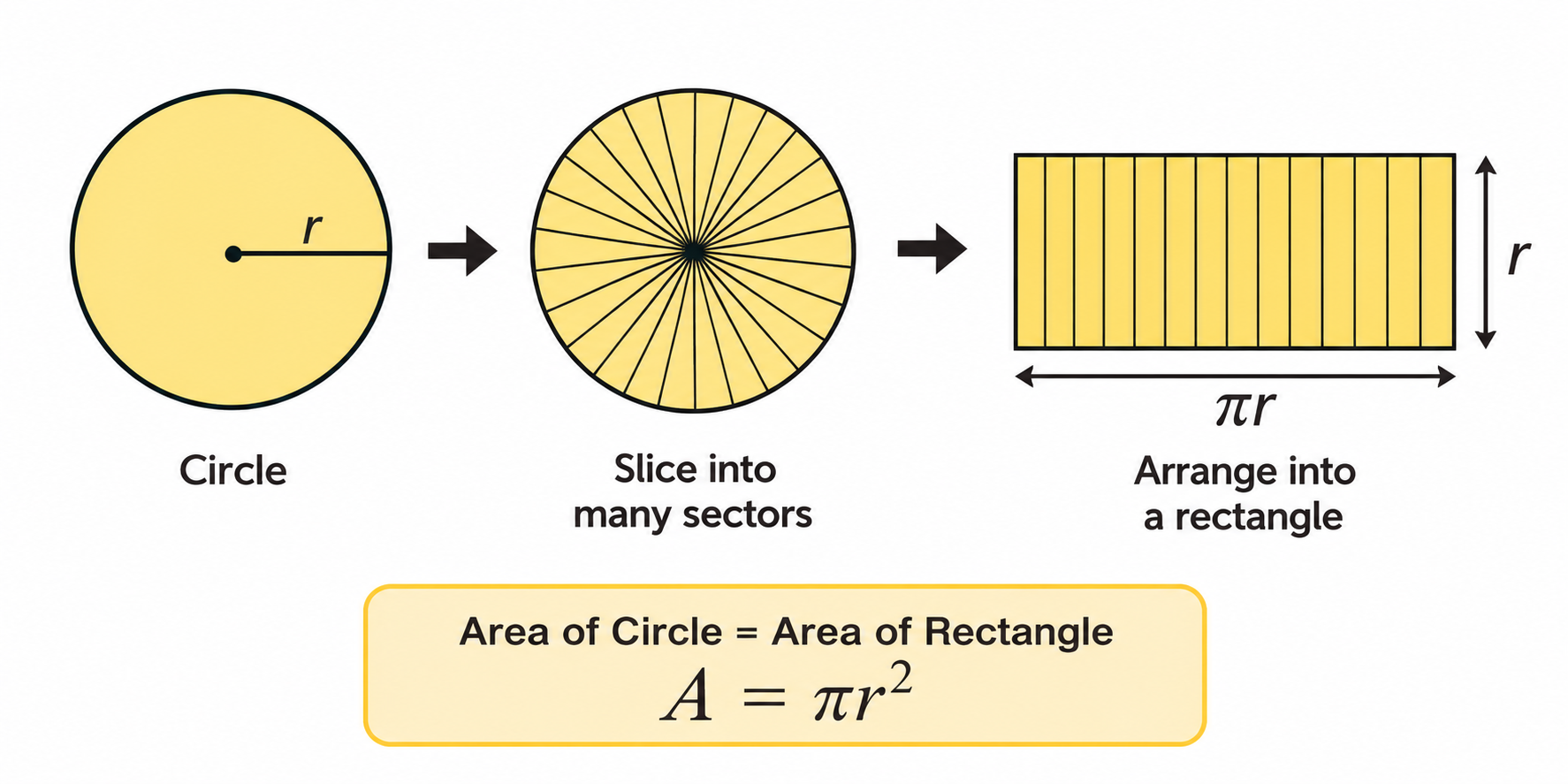
• Example: Finding the area of a circle by slicing it up and arranging those slices into a rectangle.

2. Approximation (“Tending To”):

• Example: $X \to 2$ means X is extremely close to 2 (like 1.999999 or 2.000001), not necessarily the exact integer.

3. Geometry Meets Algebra:
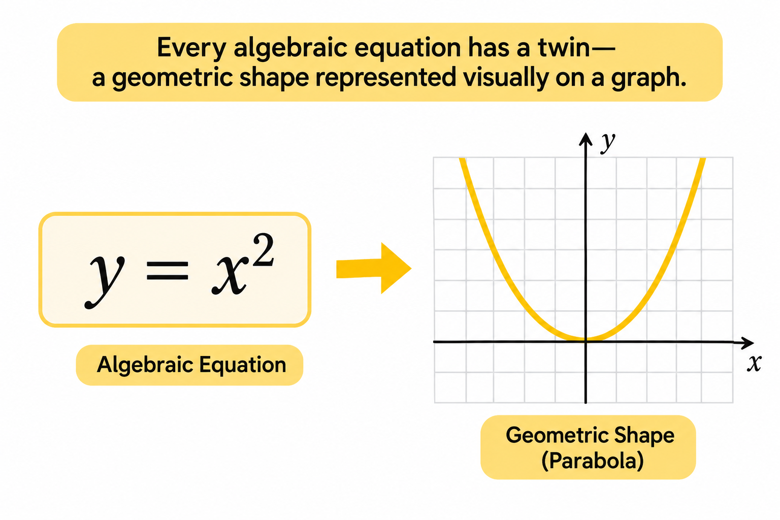
   Every algebraic equation has a twin—a geometric shape represented visually on a graph.

4. The Idea of the Slope:
   Slope measures steepness (Vertical Distance / Horizontal Distance). Depending on the graph, slopes can be constant (straight lines) or variable (curves).

5. Mathematical Representation:
   The formal formula for slope is expressed as: $\text{Slope} = \frac{\Delta y}{\Delta x}$

1. Introduction to Differentiation

1.0 Core Concept: Finding the slope of a graph.

• Differentiation: The mathematical process of calculating a derivative.
• Derivative: The resulting function

1.1 Slope of a Line

• Basic Formula: $$\text{slope} = \frac{\Delta y}{\Delta x} = \frac{y_2 - y_1}{x_2 - x_1}$$
• Using Function Notation ($f(x)$): Replacing $y$ with $f(x)$ gives the slope function between two points: $$\text{slope} = \frac{f(x_2) - f(x_1)}{x_2 - x_1}$$
• Secant Line: This represents the slope of a secant line connecting two points on a curve.

1.2. From Secant to Tangent (Derivatives)

• Approximation: On a curve, a secant line approximates the slope between two points.
• Tangent Line: When the distance between the two points approaches zero ($h \to 0$), the secant line becomes a tangent line.
• The slope of this tangent line represents the instantaneous rate of change at a single point, which is the derivative ($f'(x)$).

1.3. The Derivative Formula:

1.4 Example: Finding the Derivative of $f(x) = x^2$:

Problem: Find the slope of the tangent line to $f(x) = x^2$ at any point $x$.

Step-by-step Solution using the limit definition:

Set up the formula:

Expand the numerator:

Simplify terms:

Evaluate the limit as $h \to 0$:

(The slope of the tangent line to $f(x) = x^2$ at any point $x$ is $2x$.)

• Secant line: Line passing through 2 points on curve.
• Tangent line: Line passing thriugh the curve at one point without crossing it.

1.5 Derivative Rules:
Derivative rules help make calculations easier without always needing the long limit definition.

A. Power Rule & Constant Rules:

• Power Rule:

• Constant & Linear Rules:

Examples with Special Powers:

• Negative Power: $\frac{d}{dx}(x^{-2}) = -2x^{-3}$

• Fractional Power: $\frac{d}{dx}(x^{4/3}) = \frac{4}{3}x^{\frac{4}{3} - 1} = \frac{4}{3}x^{1/3}$

• Polynomial Example: If $f(x) = x^4 + 2x^3 + x^2 + 4x - 1$, then $f'(x) = 4x^3 + 6x^2 + 2x + 4$

B. Product Rule:
Used when finding the derivative of the product of two functions ($u$ and $v$).

• Formula:$\frac{d}{dx}(u \cdot v) = u \cdot \frac{dv}{dx} + v \cdot \frac{du}{dx}$

• Example: Find derivative of $f(x) = (x^2 + 1)(x^3 + x + 5)$
  Apply rule: $f'(x) = (x^2 + 1)(3x^2 + 1) + (x^3 + x + 5)(2x)$
  Expand: $f'(x) = 3x^4 + 3x^2 + x^2 + 1 + 2x^4 + 2x^2 + 10x$
  Simplify: $f'(x) = 5x^4 + 6x^2 + 10x + 1$

C. Quotient Rule:
Used when finding the derivative of a division of two functions ($\frac{u}{v}$).

• Formula: $\frac{d}{dx}\left(\frac{u}{v}\right) = \frac{v \frac{du}{dx} - u \frac{dv}{dx}}{v^2} \quad (\text{where } v \neq 0)$

• Example: Find derivative of $f(x) = \frac{x^2 + 1}{3x - 2}$
  Apply rule: $f'(x) = \frac{(3x - 2)(2x) - (x^2 + 1)(3)}{(3x - 2)^2}$
  Simplify numerator: $\frac{6x^2 - 4x - 3x^2 - 3}{(3x - 2)^2} = \frac{3x^2 - 4x - 3}{(3x - 2)^2}$

D. Chain Rule (Outside-Inside Rule):

• Formula: $\frac{dy}{dx} = \left(\text{derivative of outside function, keeping inside alone}\right) \cdot \left(\text{derivative of inside function}\right)$

• Example: Find derivative of $y = (3x + 7)^7$
  Apply rule: $\frac{dy}{dx} = 7(3x + 7)^6 \cdot (3)$
  Simplify: $\frac{dy}{dx} = 21(3x + 7)^6$

2. Partial Derivatives

• When a function has more than one input, like $f(x, y)$, it describes a surface rather than a curve. Hill analogy: the steepness you feel depends on which way you walk.

• Partial derivatives give the slope in two specific directions:

• $\frac{\partial f}{\partial x}$: slope when you walk only along the $x$-axis ($y$ stays fixed).
  $\frac{\partial f}{\partial y}$: slope when you walk only along the $y$-axis ($x$ stays fixed)

• The core rule, Pick one variable, freeze the rest, and differentiate as if it were a single-variable problem.

2.0 Example: $f(x, y) = x^2 + 3xy + y^2$

• Derivative with respect to $x$ (treat $y$ as a constant):

$x^2 \to 2x$
$3xy \to 3y$, because $3y$ is just a constant multiplier on $x$, like the 5 in $5x$
$y^2 \to 0$, because it contains no $x$, so it’s a constant and constants differentiate to 0.

$\frac{\partial f}{\partial x} = 2x + 3y$

• Derivative with respect to $y$ (treat $x$ as a constant):

$x^2 \to 0$
$3xy \to 3x$
$y^2 \to 2y$

$\frac{\partial f}{\partial y} = 3x + 2y$

2.1 Application: Neural Networks

• “If we change one weight, how does the loss change?”

• A neural network has a loss function that measures how wrong its predictions are, and that loss depends on thousands or millions of weights $w_1, w_2, \dots$. The partial derivative $\frac{\partial L}{\partial w_i}$ tells you how much the loss changes if you tweak just that one weight.

• Collecting all of these partial derivatives gives the gradient. Training (gradient descent) repeatedly nudges each weight in the direction that lowers the loss.

3. Numerical vs Analytical derivative

• There are 2 ways to compute derivaties:
  1. Analytical: Derive the exact formula by hand using calculus rules.
  2. Numerical: Calculate, using the formula with a tiny h (e.g. h = 0.001)

Here is a clear and structured explanation of your notes, which provide a fantastic intuitive breakdown of the Hessian matrix, second-order derivatives, and how they apply to optimization and Machine Learning.

4. Hessian Matrix

• Gradient ($\nabla f(x)$): Represents the 1st derivative. It tells you the slope of the function at any given point (the steepness and the direction of the steepest ascent/descent).

• Hessian Matrix ($H$): Represents the 2nd derivative ($f_{xx}$). It tells you the shape of the landscape (curvature)—how the slope itself is changing.

4.1. The Hessian Matrix Structure (For 2 Variables: $x$ and $y$)

For a function of two variables, $f(x, y)$, the Hessian is a $2 \times 2$ matrix of second-order partial derivatives:

$H = \begin{bmatrix} f_{xx} & f_{xy} \\ fyx & f_{yy} \end{bmatrix}$

• $f_{xx}$: Rate of change of the slope in the $x$-direction.

• $f_{yy}$: Rate of change of the slope in the $y$-direction.

• $f_{xy}$ (and $f_{yx}$): Mixed partial derivatives—how the slope in the $x$-direction changes as you move in the $y$-direction (and vice versa).

4.2 Example Analysis (“The Bowl”):

Looking at your example function $f(x, y) = x^2 + y^2$:

1. First derivatives: $f_x = 2x$, $f_y = 2y$

2. Second derivatives: $f_{xx} = 2$, $f_{yy} = 2$, $f_{xy} = 0$

3. Hessian Matrix:

$H = \begin{bmatrix} 2 & 0 \\ 0 & 2 \end{bmatrix}$

Because both diagonal entries ($2$ and $2$) are positive and constant, the surface curves upward in all directions like a bowl (a shape representing a local minimum).

4.3. Classifying Critical Points (The Determinant Test) :

At a point where the gradient is zero (flat spot), the Hessian helps determine what kind of point it is by computing the determinant $D$:

$D = f_{xx} \cdot f_{yy} - (f_{xy})^2$

4.4. Why Derivatives Matter & Why We Use Higher Orders

• 1st Derivative: Tells you the slope.

• 2nd Derivative: Tells you the curvature and helps with optimization (knowing how fast you need to accelerate or brake).

• 3rd Derivative: Used in fields like mechanical engineering (e.g., designing smooth elevator transitions so passengers don’t experience abrupt jerks in acceleration, known as jerk).

4.5. Why the Hessian Matters in Machine Learning

Standard Gradient Descent (GD) only looks at the slope (1st derivative). Newton’s Method, however, leverages the Hessian matrix to optimize weights more intelligently:

• Standard Gradient Descent update:

$w_{\text{new}} = w_{\text{old}} - \text{learning rate} \times \text{gradient}$

• Newton’s Method update:

$w_{\text{new}} = w_{\text{old}} - H^{-1} \times \text{gradient}$

Key Intuition on Curvature:

• In steep directions (high curvature/large Hessian), Newton’s method takes smaller steps to avoid overshooting.

• In flat directions (low curvature/small Hessian), it takes larger steps to move faster through flat regions.

Production Reality:

While Newton’s method is mathematically powerful, computing and inverting a massive Hessian matrix for millions of neural network weights is computationally expensive. That is why Adam (Adaptive Moment Estimation) is typically used as the default optimizer in deep learning, striking a balance by approximating adaptive learning rates efficiently.

Final summary note highlights this evolution:

$\text{ADAM} > \text{Newton} > \text{GD}$

5. Chain Rule:

• The Chain Rule is a method in calculus that helps us find the derivative of a function that is inside another function.

• A simple example - Real-life intuition: Imagine this:

• You press the accelerator in a car.
• The engine speed (RPM) increases.
• The car’s speed increases because of the engine speed. Here, one thing affects another thing, which affects something else.

The chain rule helps us calculate how changes pass through a chain of dependent variables.

• Why is this important in Machine Learning?

Input(x) -> layer1 -> layer2 -> layer3 -> Final output

A neural network has multiple layers. Each layer depends on the previous layer.

During training, we need to understand how changing a weight affects the final error (loss). The chain rule allows us to calculate this

6. Taylor Series Approximation:

Imagine you have a complicated mathematical function, and you want to calculate its value near a point. Instead of calculating the complicated function directly, you approximate it using a simple polynomial. That is the main idea behind a Taylor Series Approximation.

1. example: Suppose you want to calculate ($e^x$), where ($e$) is Euler’s number.

We know that ($e^x$) can be complicated to calculate by hand. Taylor series lets us approximate it using:

Here, $2! = 2 \times 1 = 2$, and $3! = 3 \times 2 \times 1 = 6$.

Let’s calculate ($e^{0.1}$).

Substitute (x=0.1): $e^{0.1}\approx 1+0.1+\frac{0.1^2}{2}+\frac{0.1^3}{6}$

$=1+0.1+0.005+0.000167$

$\boxed{e^{0.1}\approx1.105167}$

The actual value is approximately (1.105171). Our approximation is very close!

6.1. Why This Matters

In fields like computer vision, and machine learning optimization, computers often have to deal with complex loss functions or non-linear models where exact calculations are too computationally expensive. By using Taylor expansions (especially first-order linear approximations or second-order quadratic approximations like the Hessian), we can locally linearize or simplify complex landscapes to make gradient descent and numerical solving feasible!

These notes provide a clear, step-by-step introduction to integral calculus, moving from the basic geometric intuition of area under a curve to solving both definite and indefinite integrals using the power rule.

Here is a comprehensive breakdown of the concepts covered across your notes:

7. Integral?

• Core Concept: An integral is essentially a continuous summation. If you slice an area under a curve into infinitely thin vertical strips ($dx$) and add them all up, you get the exact area under the curve.

• Notation: Represented by the symbol $\int$, the area under a function $y = f(x)$ from a starting point to an ending point is written as:

$\text{Area} = \int y \, dx$

7.1. Area Without vs. With Integrals

• Straight-Line Graphs (No Integral Needed): For simple linear functions like $f(x) = x$, you can calculate the area under the curve using basic geometry formulas (like the area of a triangle: $\text{Area} = \frac{1}{2} \times \text{base} \times \text{height}$).

• Curved Graphs (Integral Needed): When a graph curves, geometric formulas no longer work directly because the top boundary is not a straight slope. This is where calculus and integration become necessary to sum up the infinite thin strips.

7.2. Definite vs. Indefinite Integrals

Your notes distinguish between two main types of integrals:

• Definite Integrals:

• Have lower & upper limits (numbers attached to the integral sign, e.g., $\int_{0}^{4}$).

• Result: Evaluates to a specific numerical value (representing an exact area).

• Example : Evaluating $\int_{0}^{4} x \, dx$ yields a final area of $8$.

• Indefinite Integrals:

• Do not have limits.

• Result: Yields a general function rather than a single number. Because differentiation of a constant is zero, integration of a function leaves an unknown vertical shift, so we must add a constant of integration ($+ C$) where $C \in \mathbb{R}$ (real numbers).

7.3. Key Integration Rules & Examples Solved

The Power Rule for Integration:

$\int x^n \, dx = \frac{x^{n+1}}{n+1} + C \quad (\text{for } n \neq -1)$

Walkthrough of Examples:

1. Definite Integral Example :

$\int_{0}^{4} x \, dx = \left[ \frac{1}{2}x^2 \right]_{0}^{4}$

• Plugging in the upper limit ($4$) and lower limit ($0$):

$= \left(\frac{1}{2}(4)^2\right) - \left(\frac{1}{2}(0)^2\right) = 8 - 0 = 8$

2. Indefinite Integral with a Coefficient :

$\int 4x^6 \, dx = \frac{4x^{6+1}}{6+1} + C = \frac{4}{7}x^7 + C$

3. Polynomial Integration :

$\int (x^2 + 2x - 7) \, dx$

• Integrate term by term:

• $\int x^2 \, dx = \frac{x^3}{3}$

• $\int 2x \, dx = \frac{2x^2}{2} = x^2$

• $\int -7 \, dx = -7x$ (using the rule $\int c \, dx = cx$)

• Final Answer: $\frac{1}{3}x^3 + x^2 - 7x + C$

4. Integration with Constants as Parameters :

$\int \left(8ax^4 + \frac{1}{7}x^3\right) dx$

• Treating $a$ as a real number constant:

• $\int 8ax^4 \, dx = \frac{8a x^5}{5}$

• $\int \frac{1}{7}x^3 \, dx = \frac{1}{7} \cdot \frac{x^4}{4} = \frac{1}{28}x^4$

• Final Answer: $\frac{8a}{5}x^5 + \frac{1}{28}x^4 + C$ (where $a, C \in \mathbb{R}$)

8. Multivariate Chain Rule — Explained Simply

The multivariate chain rule is a method in calculus for finding how a function changes when it depends on multiple variables, and those variables are also changing.

Think of it as: When one thing changes, it affects multiple things, which together affect the final result.

8.1. First, understand the normal chain rule

Suppose:

and

Here, $y$ depends on $x$, and $x$ depends on $t$.

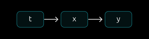
To calculate how $y$ changes with $t$:

We know:

Therefore:

8.2. Now, the multivariate chain rule

Imagine a function depends on two variables instead of one.

But both $x$ and $y$ depend on another variable $t$:

Here’s the relationship:

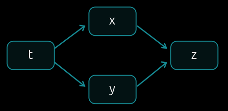
There are two paths from $t$ to $z$: through $x$ and through $y$.

When $t$ changes:

• $x$ changes, affecting $z$.
• $y$ changes, also affecting $z$.

So, to find the total change in $z$, we add the effects from both paths.

The formula is:

The symbol $\partial$ means partial derivative: differentiate with respect to one variable while treating the others as constants.

8.3. Solve the example step by step

We have:

Step 1: Find the partial derivatives.

Step 2: Find how $x$ and $y$ change with $t$.

Step 3: Apply the multivariate chain rule.

Substitute $x = 2t$ and $y = 3t$:

That’s it!

9. Jacobian Matrix

A Jacobian matrix is a table of derivatives that tells us how multiple outputs change when multiple inputs change.

Think of it as an extension of the ordinary derivative to functions with several inputs and outputs.

9.1. First, remember the derivative

Suppose:

Its derivative is:

At $x = 3$:

This means when $x$ increases by a tiny amount, $y$ increases approximately 6 times as much.

But what happens when a function has two inputs and two outputs?

That’s where the Jacobian comes in.

9.2. Imagine a machine with two inputs

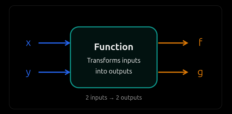
Suppose the machine has these functions:

Notice:

• Inputs: $x, y$
• Outputs: $f, g$

We want to know how each output changes when we change either input.

9.3. Calculate the Jacobian matrix

First, calculate the partial derivatives.

For $f(x,y) = x^2 + y$:

For $g(x,y) = xy$:

Now arrange these derivatives into a matrix:

Substitute the derivatives:

That’s the Jacobian matrix!

Each row represents one output, and each column represents one input.

9.4. Let’s calculate with real numbers

Suppose $x = 2$ and $y = 3$.

Here’s what it means:

So if we increase $x$ by a very small amount, $f$ changes approximately 4 times that amount, while $g$ changes approximately 3 times that amount.

9.5. Visual intuition: What does the Jacobian actually do?

Imagine drawing a tiny square on a rubber sheet. A mathematical transformation stretches, rotates, or shears that sheet.

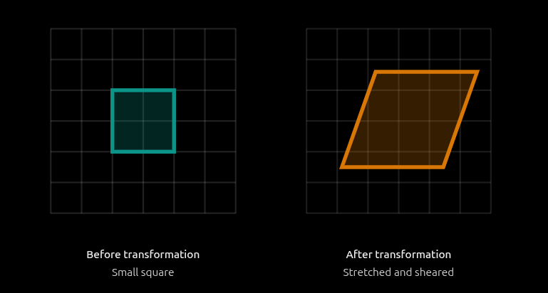
The Jacobian tells us approximately how the transformation stretches, rotates, or shears a tiny region near a point.

This is especially useful in computer graphics, robotics, physics, and machine learning.

9.6. Jacobian vs Gradient vs Hessian

Important connection to machine learning: The Jacobian is used in backpropagation, alongside the multivariable chain rule, to calculate how changes in model parameters affect outputs.

🎉 Congrats, you have completed Calculus Part-1.